Product life-cycle assessments (LCAs) and corporate greenhouse gas (GHG) inventories are notoriously time-consuming, and often prohibitively expensive for many companies and organizations. But carbon footprinting of products and companies is more important than ever. If we are going to bend the emissions curve in this critical decade, emissions accounting must become as commonplace as financial accounting.
Our stated mission at CleanMetrics is to make carbon footprinting fast, easy, affordable and scalable. Our latest service offering does exactly that by streamlining, standardizing and automating the process – all without sacrificing quality and rigor. We are calling it Rapid Carbon Footprinting ™ (RCF).
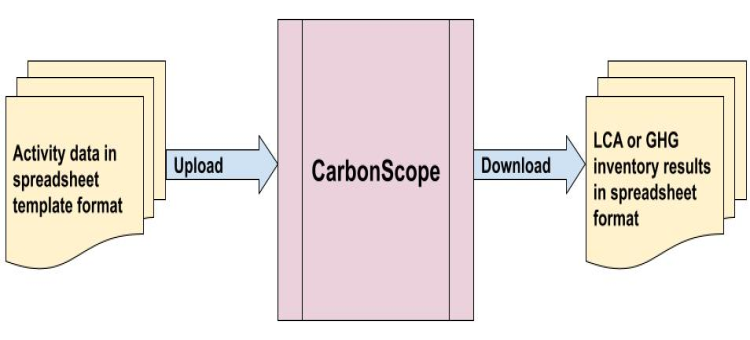
RCF uses standardized templates for both product LCAs and corporate GHG inventories. Customers enter their product or corporate activity data in our Excel templates. We upload the filled out templates into CarbonScope and download results that can be emailed to customers after an internal technical review.
Turnaround times can be as short as 2-3 business days, and the cost per product or corporate location is under $800. This is an order-of-magnitude reduction in time and cost compared to industry average. With volume discounts, RCF is highly scalable for footprinting multiple products or complex corporate structures with many locations.
Product LCAs using RCF
Product LCA Template
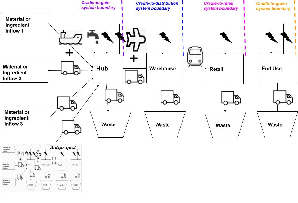
Product LCAs are based on a standard template of a product life cycle as illustrated above. Various system boundaries are possible, such as cradle-to-gate, cradle-distribution, cradle-to-retail and cradle-to-grave. The data options and choices available in the template are tied to our extensive life-cycle inventory (LCI) database.
Customers fill out an Excel template that matches this life-cycle perspective, and the results are delivered in another spreadsheet. Here is a simple example:
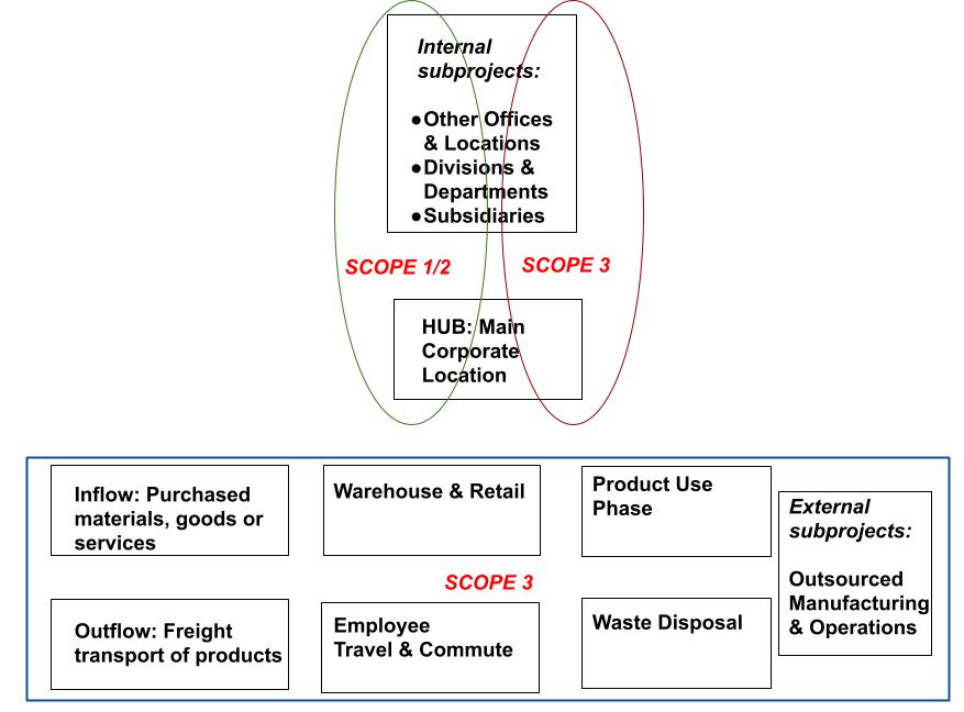
Corporate and organizational GHG inventories are based on a standard template of an organization’s activities as illustrated above. Corporate structures of varying complexity can be modeled, such as: multiple locations, divisions, departments, subsidiaries, and outsourced operations. We use a hybrid methodology – combining process-based and economic input-output based LCI data – for fast and efficient modeling.
Customers fill out an Excel template that matches this organizational perspective, and the results are delivered in another spreadsheet. Here is an example:
The activity data templates require Excel macros for full functionality. Both the LCA and the GHG inventory templates are available for download as Excel files.
We are seeing a surge of interest in life cycle assessments (LCAs) for determining the carbon footprints of food products. In many food LCAs, attention turns rather quickly to the agricultural practices used to produce the ingredients. This is especially the case with producers of processed food products who source ingredients grown using organic and/or regenerative methods. We summarize here what is in our soil model as implemented in FoodCarbonScope and CarbonScopeData, how we model soil dynamics and what the standards say about all this.
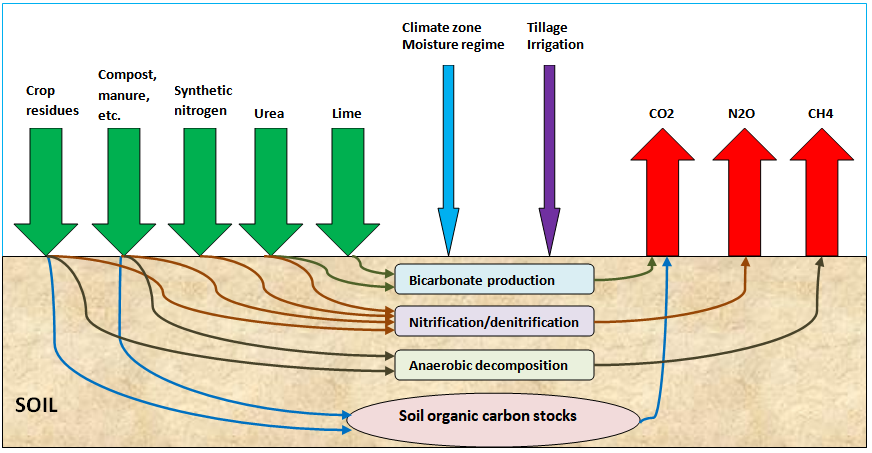
The diagram above captures the flow of key inputs into the soil and the resulting emissions of greenhouse gases (GHGs) as well as sequestration of soil organic carbon. The inputs of interest are synthetic fertilizers, organic fertilizers and soil amendments, and crop residues. The soil model basically tracks, to a first-order approximation, what happens to the nitrogen and carbon in these various inputs. The GHGs that are released as a result of these inputs, as well as due to land management practices and climatic conditions, are nitrous oxide (N2O), carbon dioxide (CO2) and methane (CH4).
How we model soil dynamics
Changes in soil organic carbon
We use the IPCC tier 1 parameters (see discussion in the last section) to estimate changes to soil organic carbon (SOC) stocks in croplands. These parameters are a function of land management practices (tillage method, carbon inputs to soil), climate zone, moisture regime, and soil type. The default time period for stock changes is nominally 20 years and management practice is assumed to influence stocks to a depth of 30 cm. Soil carbon is considered to be in steady state until there is a significant land-use change (such as a conversion from grassland to cropland) or management change (such as a conversion from conventional cropland to organic cropland) that changes the soil carbon stocks.
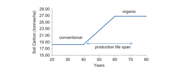
When such a change occurs, the soil carbon is assumed to reach steady state again after 20 years under the new land-use or management practice. During this 20-year transition period, soil carbon may be increasing or decreasing each year as illustrated below, thus increasing or decreasing the total greenhouse gas emissions and the product carbon footprint during that period. When soil carbon is in steady state, it does not contribute to net emissions in agricultural systems.
Regarding the question of why a steady-state organic farming system does not get credit for the potentially higher level of carbon (relative to a conventional farming system) already accumulated in the soil: The addition of organic matter balances the carbon that is naturally oxidized away from the top layers of the soil, so in an ideal steady-state system, the SOC level remains constant and the net change in soil carbon is zero. LCA models account for this net change and a production system can take credit in the years that this net change > 0. Likewise, if we allowed the organic system to degrade by not adding sufficient organic matter to the soil for a few years, it would result in a new transition with net change < 0, resulting in a higher carbon footprint for those years. So maintaining a steady-state organic system avoids this higher carbon footprint — and that in a nutshell is the benefit of continuously adding organic matter to the soil. That benefit is already reflected in the stable carbon footprint of a steady-state organic system.
The 20-year transition period itself is not a critical parameter. Our tools allow the user to set this to any reasonable value. The more important issue is the magnitude of changes to the SOC stocks over the transition period. There can be wide variability and crop specificity in field measurements of soil carbon stocks, and the tier 1 parameters provide useful estimates of typical SOC changes while avoiding the complexity and data collection effort associated with tier 2/3 models.
Nitrous oxide emissions due to nitrogen inputs
Synthetic nitrogen fertilizers (nitrate, ammonia, ammonium or urea) and organic nitrogen sources (compost, manure or crop residues) produce direct N2O emissions from the soil through the nitrification-denitrification process mediated by soil bacteria. In addition, indirect N2O emissions result from the volatilization and redeposition of NH3/NOx, and through leaching and runoff of nitrogen.
We calculate both direct and indirect N2O emissions based on the amounts of synthetic and various organic nitrogen sources added to the soil each year, as well as due to nitrogen from crop residues and distinguishing between typical agricultural soils and flooded rice fields. We also make an adjustment for legumes to account for the excess ammonium that may leak from nitrogen-fixing root nodules and ultimately escape to the atmosphere as N2O.
Carbon dioxide emissions due to lime and urea
CO2 is released directly due to the application of lime and urea to agricultural soils. Liming is used to reduce soil acidity and improve plant growth. When carbonates such as limestone (CaCO3) are added to soils, they dissolve and release bicarbonate (HCO3-) which evolves into CO2 and water. When urea is applied as a fertilizer, it releases bicarbonate which again evolves into CO2 and water. We calculate these CO2 emissions based directly on the amounts of lime and urea applied each year to a given land area.
Methane emissions from rice fields
Anaerobic decomposition of organic material in flooded rice fields produces CH4. We calculate the annual amount of CH4 emitted from a given area of rice as a function of the crop growth period (measured in days), irrigation method (such as continuously or intermittently flooded), and organic and inorganic soil amendments (such as straw, compost and/or manure).
What the standards say
IPCC guidelines
The IPCC guidelines for national greenhouse gas inventories provide the most detailed and standardized guidance available for calculating soil carbon emissions and sequestration, N2O emissions from soils, and CH4 emissions from soils. Given that the current product carbon footprint standards do not provide detailed guidance on these topics but defer to IPCC in general, our methodology for modeling soil dynamics is based almost entirely on the IPCC guidelines.
There are three tiers of methodology in the IPCC guidelines. We have found the tier 1 methods to be the most appropriate for LCA models used to compute product carbon footprints. Given the time and cost constraints in most LCA projects, as well as the sheer difficulty involved in obtaining country-specific data or field measurements, we use tier 1 methods as a practical default unless higher tier data are readily available.
Here is a brief description of the three tiers:
Tier 1 methods are designed to be the simplest to use, for which equations and default parameter values (e.g., emission and stock change factors) are provided by IPCC. Country-specific activity data are needed.
Tier 2 can use the same methodological approach as Tier 1 but applies emission and stock change factors that are based on country- or region-specific data.
At Tier 3, higher order methods are used, including comprehensive field sampling repeated at regular time intervals and/or GIS-based systems of age, class/production data, soils data, and land-use and management activity data, integrating several types of monitoring.
Product carbon footprint standards
Neither of the two leading product carbon footprint standards, PAS-2050 and the GHG Protocol Product Standard, requires soil carbon changes (due to changes in management practices such as tillage) to be included in the carbon footprint of agricultural products. The default is to exclude it, but both standards provide for ways to include it (in the case PAS 2050, it can be included in accordance with the standard’s supplementary requirements). Both standards do require direct land use change (such as conversion from grassland to cropland) to be included per IPCC guidelines, but indirect land use change is not included in the carbon footprints. Our methodology is consistent with both standards, and we do include the effects of both land management practices and direct land use changes.
PAS 2050 requires non-CO2 emissions (N2O, CH4) from soils to be assessed using the highest tier approach set out in the IPCC guidelines or the highest tier approach employed in the country in which the emissions are produced. The Product Standard does not provide specific guidance on this. Our methodology takes a compromise position here and defaults to using the IPCC tier 1 parameters to calculate these soil emissions.
Carbon registries
The methodology described here generally aligns with the principles developed by carbon registries (for example, the Climate Action Reserve’s Soil Enrichment Protocol) for allocating carbon credits based on soil carbon sequestration.
An annual corporate greenhouse gas (GHG) emissions inventory – if done correctly – can tell you exactly where your company or organization stands as far as its climate impact and how that changes over time. It is a starting point for serious climate action that could ultimately include switching to green electricity, cutting transport emissions, using lower-emissions materials, reducing waste and purchasing high-quality carbon offsets.
But GHG inventories are notoriously time-consuming and difficult to compile, and they often require a level of expertise that most small and medium-sized enterprises do not have. This problem was front and center in our minds as we architected and developed our new carbon modeling tool, CarbonScope. As we said in a recent Medium post: If we are going to bend the emissions curve, then a majority of businesses need to get involved, and emissions accounting must become as commonplace as financial accounting.
While CarbonScope allows for some very sophisticated modeling, we want to focus here on the simplest and quickest way to compile a corporate GHG inventory that you can put to use immediately. CarbonScope is a web app designed for interactive data input and use. To keep things simple, we will propose entering all of the activity data into a spreadsheet and then uploading it into CarbonScope. Once the data is in CarbonScope, you can switch to an interactive mode for the rest of the analysis.
This simple method uses hybrid life-cycle inventory (LCI) data under the hood:
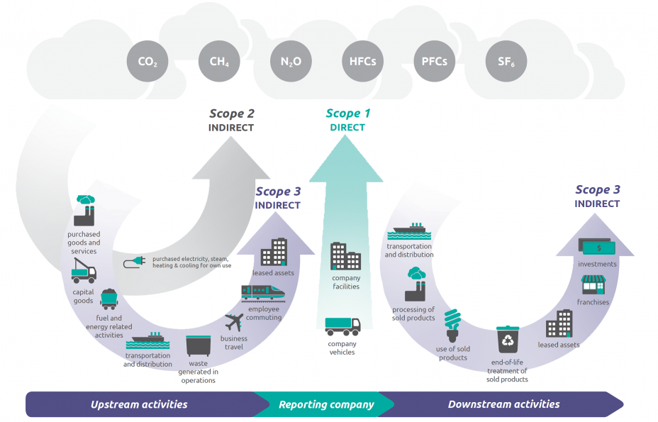
All of the emissions in scope 1 (direct fuel combustion) and scope 2 (purchased electricity) are modeled using our process LCI (PLCI) database. This is the easy part.
The wide range of emissions in scope 3 are modeled largely using our environmentally extended input-output LCI (EEIOLCI) database, which converts dollar amounts from purchase records into equivalent GHG emissions, energy use and water use based on the industry sector (or equivalently, NAICS code). This is the difficult part that we have simplified and automated to a large extent.
This hybrid method is available to companies that are using CarbonScope themselves, as well as to those that utilize our consulting services.
Compile activity data
We have an example of the activity data template here with some sample data filled in for a hypothetical company. Note that this data is for a one year period. The spreadsheet contains seven sheets:
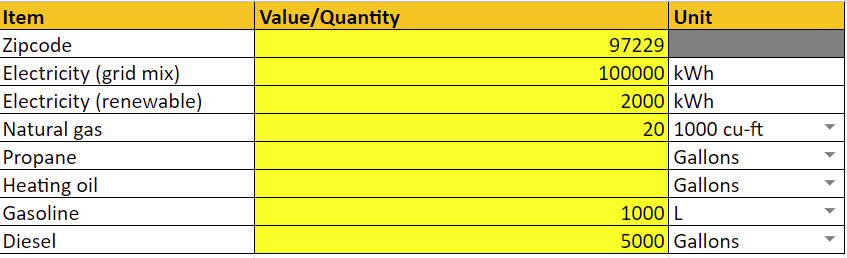
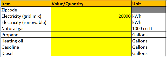
Hub: This is the company’s primary location (or it could be the location of a division, subsidiary or department). Here we would fill in the quantities of all purchased fuels and electricity, accounting for all of the scope 1 and 2 emissions (and some scope 3 emissions as well). A zipcode is required in order to find the correct electric grid emission factor in the US (alternately, you can enter a country name here for international locations). A blank zipcode defaults to US average electric grid emissions.
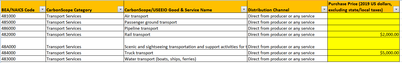
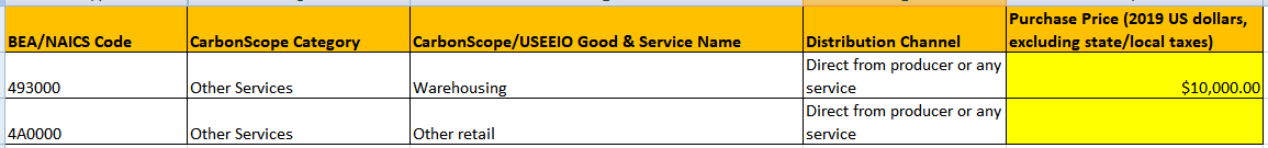
Inflow: This sheet captures all of the purchased materials, goods and services. The cool thing about this is that CarbonScope can work with dollar amounts (excluding local/state taxes) that you spent on your purchases from one or more of 385 industry sectors that cover the entire US economy. You can just convert your purchasing records into dollar amounts that can be used to represent most of the scope 3 emissions, resulting in significant savings of time and effort.
Outflow: This sheet captures all of the third-party freight transport that you paid for. It is also in dollar amounts similar to the inflow. This contributes to scope 3 emissions.
Waste: This sheet captures all of the waste management, water and wastewater services that you paid for. It is also in dollar amounts similar to the inflow. This contributes to scope 3 emissions.
Storage: This sheet captures all of the third-party warehousing or other storage of your products that you paid for. It is also in dollar amounts similar to the inflow. This contributes to scope 3 emissions.
Use Phase: This sheet captures the estimated electricity and fuels consumed in the usage of your products, or in the further processing of your products in the value chain. This contributes to scope 3 emissions. A blank zipcode defaults to US average electric grid emissions.
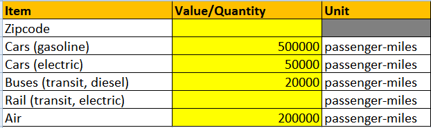
Employee Travel: This sheet captures all of the employee business travel and commuting in passenger miles on various transport modes. It is the total across the entire company (or division, department, etc.). This contributes to scope 3 emissions. A blank zipcode defaults to US average electric grid emissions.
Upload activity data
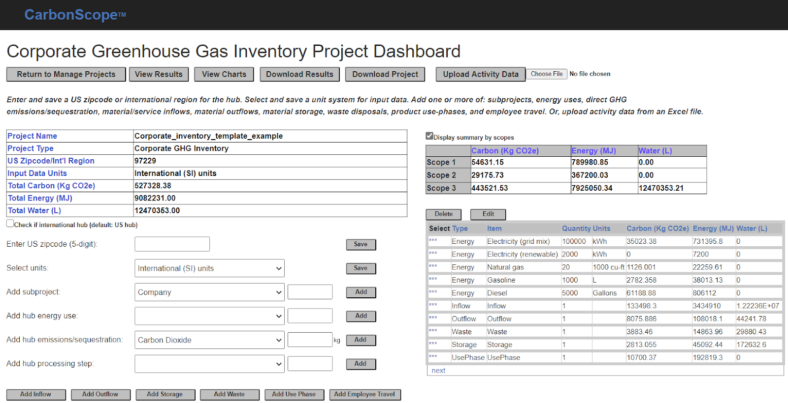
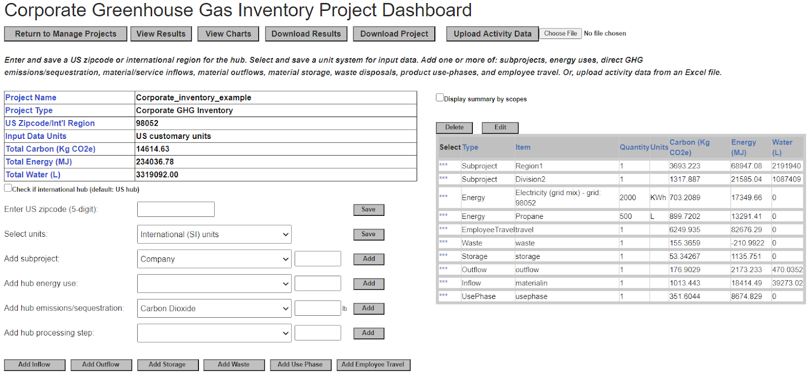
This spreadsheet with its seven sheets can be uploaded into a blank GHG inventory project in CarbonScope by selecting the Excel file and clicking “Upload Activity Data” in the CarbonScope GHG inventory dashboard. The upload will automatically populate the project and calculate all of the carbon, energy and water results in detail. At this point, all of the analysis is automatically done and summary results can be seen on the dashboard as shown below. It is as simple as that.
Note: If the company has multiple locations, divisions or subsidiaries that need to be modeled separately, you would need to fill out one copy of the spreadsheet for each of these and upload each spreadsheet into a separate GHG inventory project. Then, you would instantiate these other projects as subprojects within the GHG inventory project for the main location or the company headquarters as shown below.
View and download results
The full GHG inventory results can be downloaded by clicking “Download Results” on the dashboard. You can see the results for the above hypothetical example here. You can slice and dice the results as needed, and create your own custom reports.
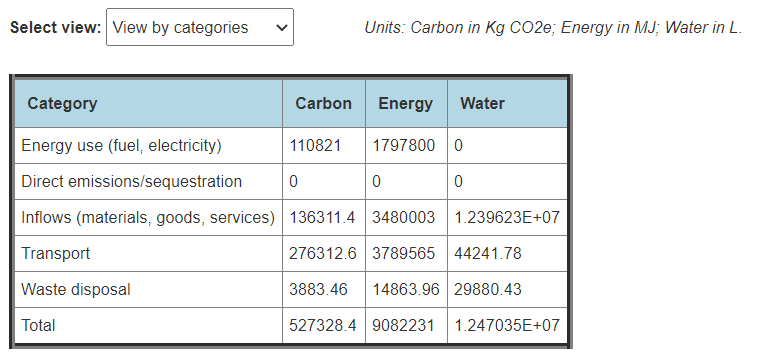
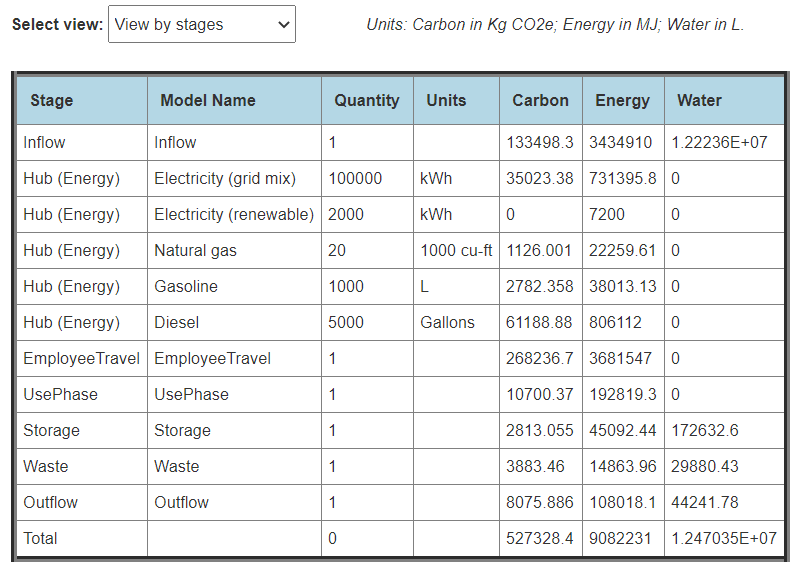
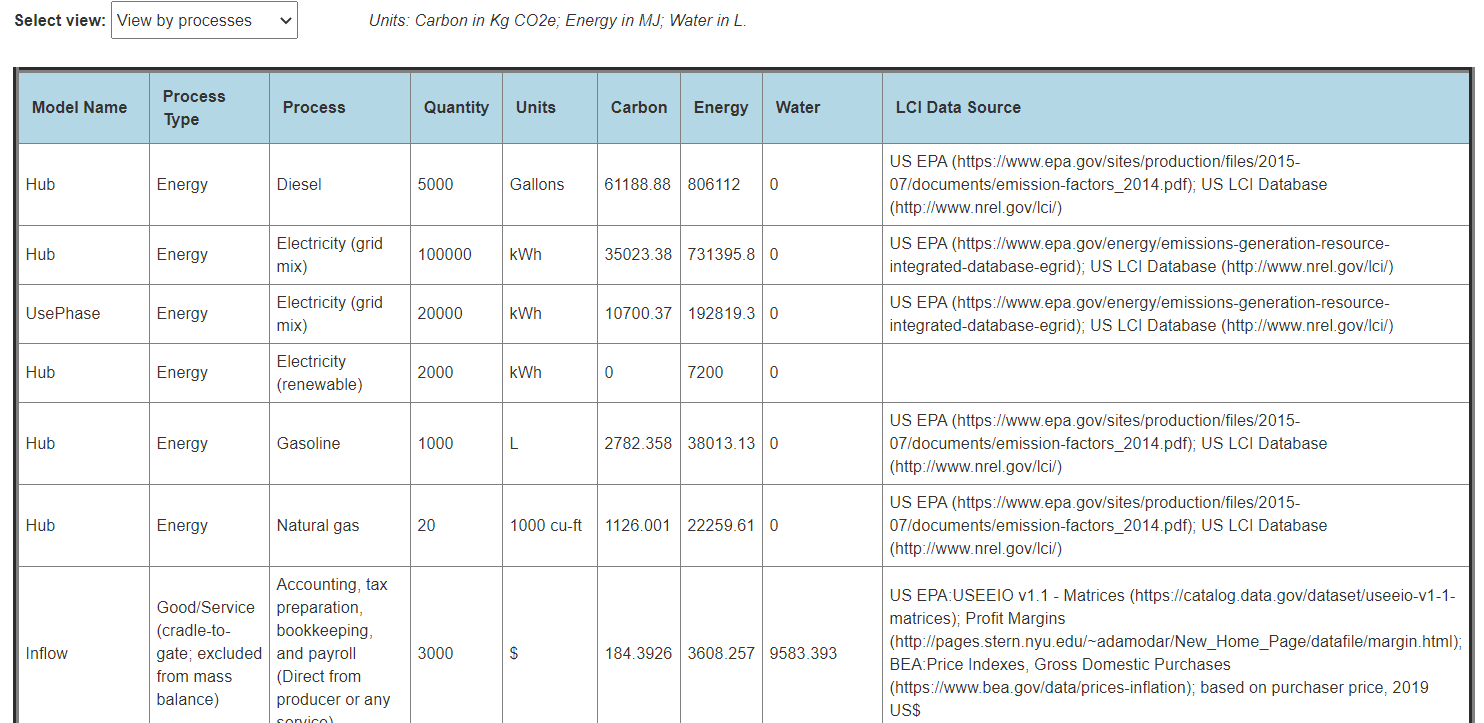
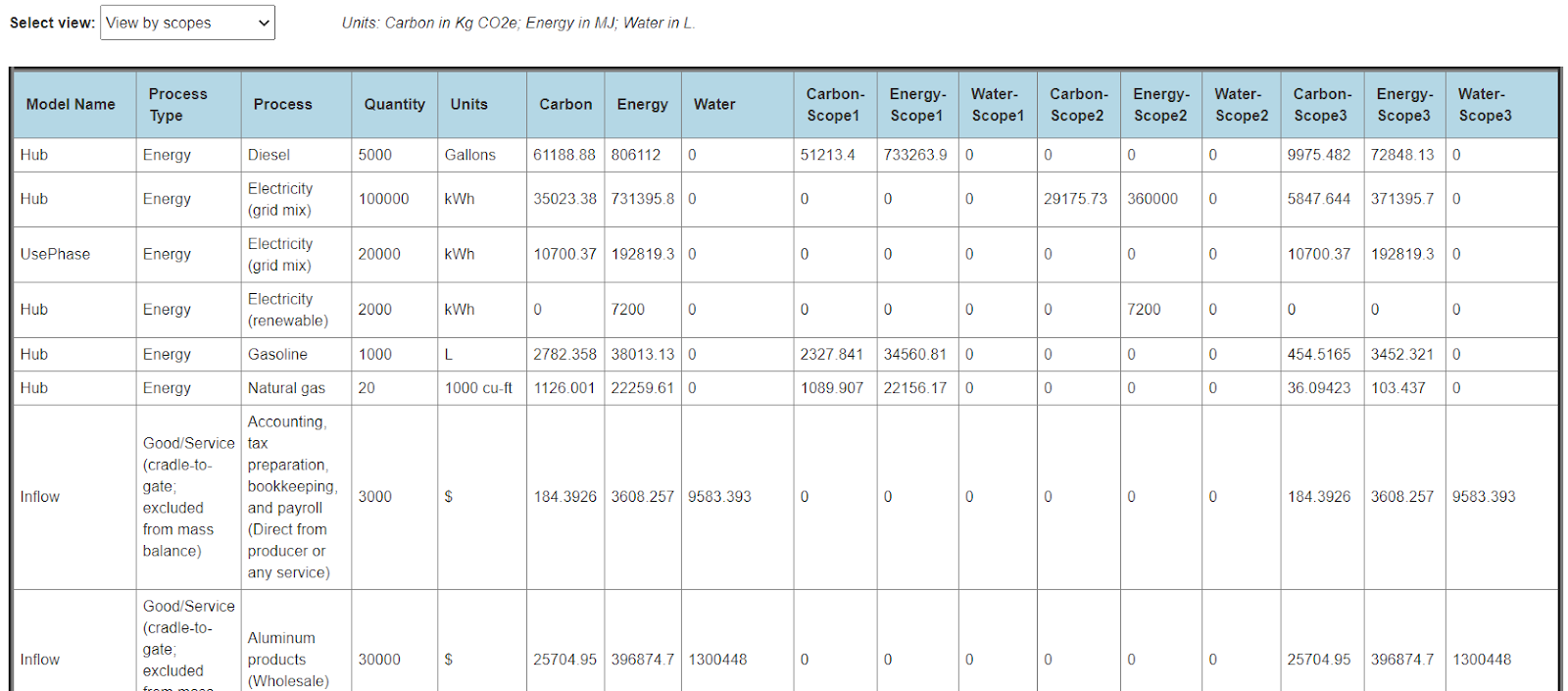
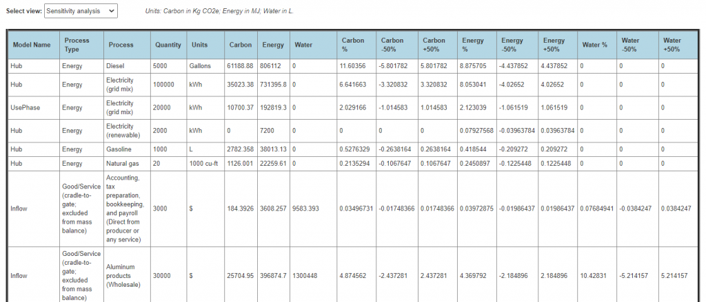
The same basic results can be viewed online by clicking “View Results” (to view as tables) or “View Charts” (to view as charts) on the dashboard and then selecting the desired “view” in the new browser tab that opens up. The results can be viewed by category, stages, processes or scopes as shown below. A sensitivity analysis table is also available.
View by categories ______________________________________________________________________View by stages ______________________________________________________________________View by processes _____________________________________________________________________View by scopes _____________________________________________________________________Sensitivity analysis ______________________________________________________________________
Correct usage of the hybrid methodology
The hybrid methodology outlined here — combining PLCI (for accurate scope 1/2 emissions and some scope 3 emissions) and EEIOLCI (for 100% coverage of most scope 3 emissions) — can be very effective in compiling corporate GHG inventories.
A limitation of EEIOLCI is that it cannot be used for evaluating the relative impacts of process improvements or material substitutions within an industry sector, or for comparing the environmental impacts of two similar products, due to the data aggregation by industry sector.
This hybrid methodology can be used to quickly establish a baseline GHG inventory and can help screen for hot spots that may require more attention. Emission reduction targets can be set immediately for scopes 1 and 2 in accordance with Science Based Targetsor other reduction plans. The inventory results can also be used directly to purchase high-quality carbon offsets as part of a broader corporate climate strategy to address all emission scopes.
With the sensitivity analysis that CarbonScope performs automatically, it is straightforward to identify the scope 3 items that the GHG inventory is most sensitive to. Based on this, some of the scope 3 items (especially the inflows of goods and services into the company/organization) could be selectively modeled using PLCI in a second iteration for more accuracy as well as to evaluate process improvements or material substitutions in order to set and achieve scope 3 emission reduction targets. Alternately, it might be useful to look at categories like employee travel for possible scope 3 emission reductions while keeping the convenient EEIOLCI modeling for inflows.