The Intergovernmental Panel on Climate Change estimates that plant-based diets could free up several million square miles of land and reduce global greenhouse gas (GHG) emissions by up to eight billion tonnes per year by 2050. There are, in fact, more immediate opportunities given the rapid market acceptance of plant-based meats. Hungry Planet, a producer of chef-crafted plant-based meats, and CleanMetrics teamed up to quantify this potential.
It is well known that plant-based foods have a much smaller environmental footprint than conventional meats. However, most of these comparisons (including past studies conducted by CleanMetrics) have involved plant foods that are not direct substitutes for animal proteins. Because Hungry Planet® meats are an authentic one-to-one match for conventional meats in taste, texture, and use, the comparisons presented in this study are more relevant to the question of how food production can be made more sustainable and climate friendly without compromising taste or nutrition.
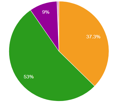
LCA results
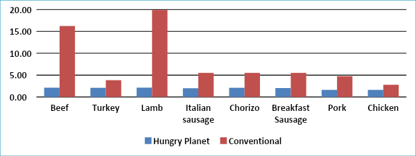
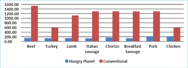
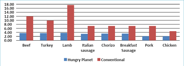
CleanMetrics used standards-based life-cycle assessments (LCAs) to evaluate eight product SKUs offered by Hungry Planet. The results showed that substituting Hungry Planet® meats for conventional meats could yield significant savings in cradle-to-gate GHG emissions, water use and land use:
Hungry Planet® meats generate 42 to 89% lower GHG emissions than conventional meats.
Hungry Planet® meats consume 62 to 91% less blue and grey water than conventional meats.
Hungry Planet® meats require 52 to 79% less agricultural land than conventional meats.
Figure 1: Comparison of Hungry Planet® vs. Conventional Meats: GHG emissions (kg CO2e/kg) Figure 2: Comparison of Hungry Planet® vs. Conventional Meats: Water use (L/kg) Figure 3: Comparison of Hungry Planet® vs. Conventional Meats: Land use (m2-yr/kg)
Putting it in context
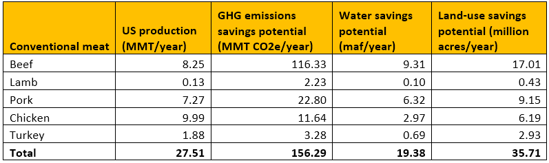
To put this in context, the table below shows hypothetical savings in GHG emissions, water use and land use that could be achieved in the US by switching to plant-based meats like Hungry Planet’s wide range of products. The total potential savings add up to as much as 25% of all US agricultural GHG emissions and water use. Moving away from conventional meats would also free up over 35 million acres of land occupied by agriculture.
Table 1: Potential savings from switching to plant-based meats in the US (production data from USDA)
There are also indirect climate benefits from switching to a plant-based diet. Wasted animal foods have 3.5 times the climate impact of plant-based foods on average due to the vast differences in the GHG emissions from production. So, switching to a plant-based diet can mitigate some of the worst climate impacts of food waste.
The choice of protein is one of the most powerful tools that we can deploy to meet climate goals and sustainability targets both at personal and corporate levels. It is also one of the easiest to act on given the wide availability of plant-based meats.
Zero-waste, upcycled, outdoor jackets customized for users by Dhana
The idea of a circular economy and closing the materials loop has been an aspirational goal for decades. But circularity as an afterthought has never really worked. We are finally starting to see products that are designed from the ground up to utilize materials that are already circulating in the economy while producing zero additional waste in the manufacturing process. An intriguing example of a circular product is the Circular Memory Jacket from Dhana, made with used clothing materials. Our life-cycle assessments (LCAs) show that these circular jackets have just 1/3 of the carbon footprint of a similar non-circular jacket and negligible water footprint – all from using 100% repurposed materials.
Systems modeled in this study
The system boundary for the LCAs is cradle to retail, starting from resource extraction and ending with the delivery of the jackets to customers. We use LCAs to compare the environmental impacts of a conventional non-circular jacket with a circular jacket from Dhana.
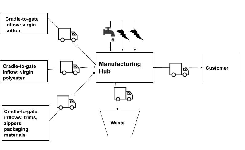
Generic, non-circular jacket production and delivery
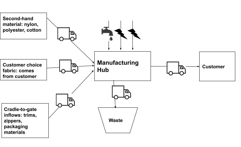
Dhana circular jacket production and delivery
The functional unit for the LCAs is one circular or non-circular jacket. The LCAs consider three life-cycle impact categories:
Carbon/GHG Emissions (climate change), kg CO2e/garment: Greenhouse gas (GHG) emissions – includes CO2, methane and nitrous oxide.
Energy, MJ/garment: Primary energy use – includes combusted and feedstock energy.
Water, L/garment: Water consumption – includes surface and groundwater used.
LCA tools and methodology
We used our carbon modeling tool, CarbonScope, to conduct the LCAs in this study. The life-cycle inventory database underlying the analysis is CarbonScopeData. The analysis was done using our Rapid Carbon Footprinting (RCF) methodology. An important part of this study is the modeling of recycled/repurposed materials in LCAs, which was done using the using the “recycled content” method.
Results and conclusion
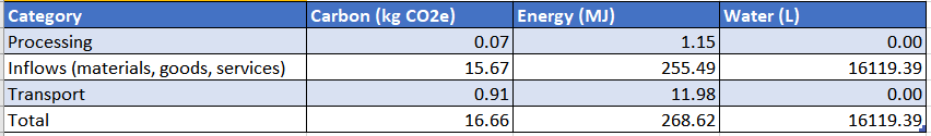
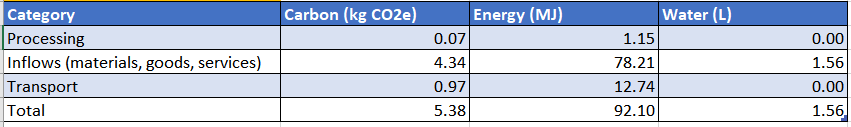
The life cycle impact assessment results below show thatthe circular jacket generates less than a third of the GHG emissions that a generic, non-circular jacket would generate from the production and transport. The emissions are dominated by the materials used to make the jackets, including cotton and polyester. Final processing (i.e., garment manufacture) and transport (both incoming and outgoing) are minor contributors.
The water footprint of a circular jacket is negligible compared to the substantial water consumption in the life cycle of a non-circular jacket, largely due to the water required to produce the virgin cotton used in the non-circular jacket.
Life cycle impact assessment for a generic, non-circular jacket made with virgin materialsLife cycle impact assessment for a Dhana circular jacket made using repurposed clothing materials
The results clearly show the significant environmental advantages that can be achieved by reusing materials that are already circulating in the economy as opposed to using virgin materials. We have seen similar results in the case of other LCAs of outerwear. The economics and logistics of recycling may be challenging in general, but the clothing sector is one where circular production looks like a practical solution that can dramatically lower environmental footprints.
——
The customer featured in this case study, Dhana Inc., is headquartered in Sausalito, California. Dhana is a certified B Corp and a pioneer in circular fashion whose mission is to connect people and planet through the medium of fashion.
Product life-cycle assessments (LCAs) and corporate greenhouse gas (GHG) inventories are notoriously time-consuming, and often prohibitively expensive for many companies and organizations. But carbon footprinting of products and companies is more important than ever. If we are going to bend the emissions curve in this critical decade, emissions accounting must become as commonplace as financial accounting.
Our stated mission at CleanMetrics is to make carbon footprinting fast, easy, affordable and scalable. Our latest service offering does exactly that by streamlining, standardizing and automating the process – all without sacrificing quality and rigor. We are calling it Rapid Carbon Footprinting ™ (RCF).
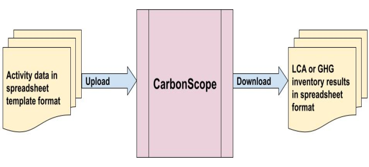
RCF uses standardized templates for both product LCAs and corporate GHG inventories. Customers enter their product or corporate activity data in our Excel templates. We upload the filled out templates into CarbonScope and download results that can be emailed to customers after an internal technical review.
Turnaround times can be as short as 2-3 business days, and the cost per product or corporate location is under $800. This is an order-of-magnitude reduction in time and cost compared to industry average. With volume discounts, RCF is highly scalable for footprinting multiple products or complex corporate structures with many locations.
Product LCAs using RCF
Product LCA Template
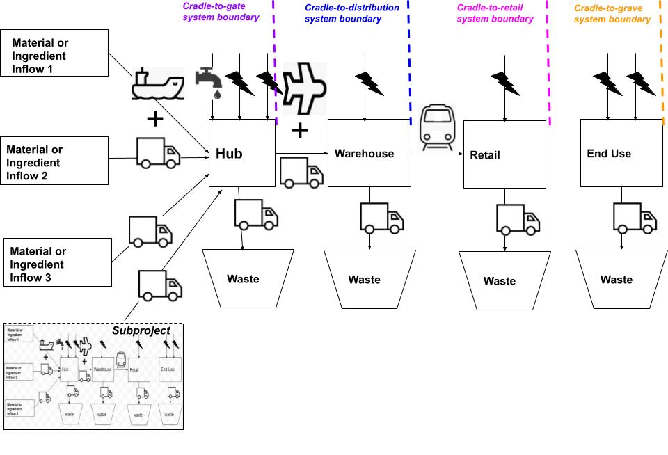
Product LCAs are based on a standard template of a product life cycle as illustrated above. Various system boundaries are possible, such as cradle-to-gate, cradle-distribution, cradle-to-retail and cradle-to-grave. The data options and choices available in the template are tied to our extensive life-cycle inventory (LCI) database.
Customers fill out an Excel template that matches this life-cycle perspective, and the results are delivered in another spreadsheet. Here is a simple example:
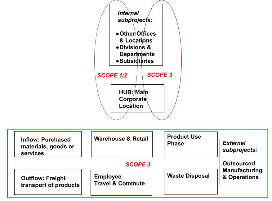
Corporate and organizational GHG inventories are based on a standard template of an organization’s activities as illustrated above. Corporate structures of varying complexity can be modeled, such as: multiple locations, divisions, departments, subsidiaries, and outsourced operations. We use a hybrid methodology – combining process-based and economic input-output based LCI data – for fast and efficient modeling.
Customers fill out an Excel template that matches this organizational perspective, and the results are delivered in another spreadsheet. Here is an example:
The activity data templates require Excel macros for full functionality. Both the LCA and the GHG inventory templates are available for download as Excel files.
A plastic maintenance shaft can cut lifecycle emissions by over 100X relative to a concrete manhole
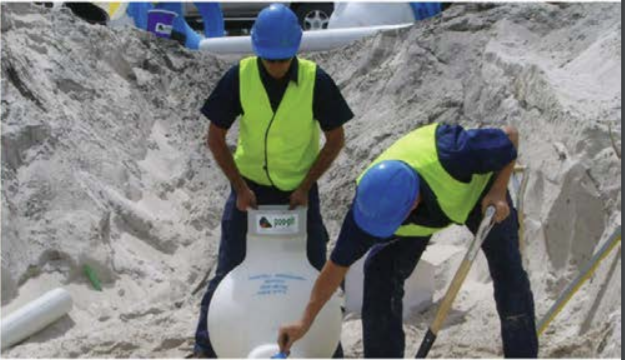
Infrastructure can be expensive, not only fiscally but also environmentally. Buildings, the most visible examples, account for nearly half of all US energy consumption in their construction and ongoing usage. Consider a less obvious but still essential infrastructure component: the ubiquitous urban sewer access point. Our life-cycle assessments (LCAs) show the dramatically large life-cycle carbon footprint savings that could be achieved by choosing plastic maintenance shafts over traditional concrete manholes.
Systems modeled in this study
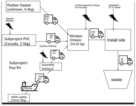
The following figures illustrate the supply chains modeled in our LCAs of the Poo Pit™ plastic maintenance shaft from Quickstream Solutions North America and the equivalent concrete manhole. The LCA system boundary is cradle-to-grave in both cases.
Figure 1 System diagram for a Poo Pit™ maintenance shaft
The Poo Pit™ is manufactured using HDPE plastic sourced from China that is then shipped to Indiana for injection molding and sub-assembly, as shown in Figure 1. Final assembly with additional PVC pipe fittings and a rubber gasket occurs in Windsor, Ontario, the company’s headquarters. The sourcing of these smaller components was unknown, so for now we make a reasonable placeholder distance (500 km) in line with other non-imported components. Although the location of install sites will vary, we set a moderate distance (200 km) from the headquarters as representative. While at 22 Kg the Poo Pit™ is sufficiently light to be carried by hand, excavators and dump trucks are needed to remove debris, haul it away, and then truck in the backfill, resulting significant usage of diesel fuel. When it is time to remove the shaft at its end of life, we assume the disposal site is a short (50 km) distance away.
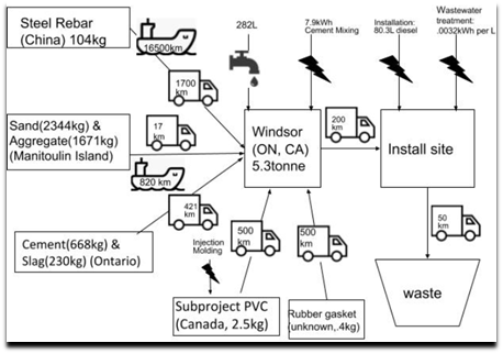
Figure 2 System Diagram for an equivalent concrete manhole
Figure 2 captures an equivalent concrete manhole. The steel rebar comes from China, but the ingredients to make concrete are sourced far more locally. To keep the comparison consistent with the Poo Pit™ we utilize identical sourcing for the PVC fittings and gasket, as well as the distances to the install and disposal sites. Given that this product is substantially heavier, at over 5 tonnes, and displaces more excavation debris, more fuel is used at the installation site. Later, we will consider the energy used for wastewater treatment.
LCA tool and LCI database
We used our carbon modeling tool, CarbonScope, to conduct the LCAs in this study. The life-cycle inventory database underlying the analysis is CarbonScopeData.
Results
The
three life-cycle impact categories CarbonScope quantifies are embodied carbon
(Kg CO2e), embodied energy (MJ) and embodied water (L), but to keep
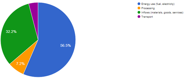
the comparisons simple, we report only embodied carbon. Figure 3 breaks down
the embodied carbon by category and shows that the majority of the 130 Kg of embodied
carbon associated with a Poo Pit™ is attributed to the energy used at
installation. The next largest impact comes from the material inflows, which
are mostly (80%) due to the HDPE plastic body, so the placeholder data for the
other components is justifiable. Transport and processing energy have only a
small part of the total share of the embodied carbon.
Figure 3 Embodied carbon from the manufacture, install, and disposal of a Poo Pit™ shaft
At 1790
Kg CO2e, the concrete equivalent has over thirteen times the carbon
footprint of a Poo Pit™. Although nearly four times as much
diesel fuel is burned during installation, installation energy is only the
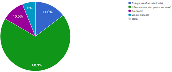
second largest impact. Figure 4 shows that material inflows have the greatest
share of the embodied carbon. In particular, Portland cement is
carbon-intensive and contributes half the total carbon footprint, and the steel
rebar contributes 15%. The other ingredients contribute little themselves
except that their massive weight leads to greater transportation emissions: Hauling
5 tonnes even short distances with efficient transport modes still takes a toll.
Figure 4 Embodied carbon from the manufacture, install, and disposal of the concrete equivalent
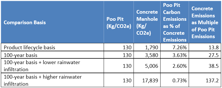
The vast embodied carbon difference between these two shafts is further magnified when one considers their lifespans. Plastic is more durable than concrete and Poo Pits™ are rated to last 100 years, twice the lifespan of their concrete equivalents. A more appropriate comparison of embodied carbon would double the carbon footprint of the concrete equivalent, and Table 1 shows that with this accounting a Poo Pit™ has less than 4% the embodied carbon of the concrete equivalent.
Furthermore, plastic’s impermeability provides another benefit over concrete: no infiltration of rainwater runoff. Rainwater seeps into concrete manholes, up to a rate of 0.8 liters per second, and must then be processed at a wastewater treatment center, requiring energy (0.00032 kWh per liter). The increased inflow associated with building out new waste management infrastructure can often restrict their development. The amount of rainwater that will need to be treated over 100 years would vary with the climate and topology of an install site.
We thus consider two scenarios in Table 1 that vary by an order of magnitude: a wet one where one of ten days has intensive rainwater infiltration, and a much dryer one where only one out of 100 days experiences such infiltration. In either scenario the treatment of the wastewater becomes the dominant contributor of carbon emissions. So once rainwater infiltration is considered a Poo Pit™ will have between 0.73% to 2.60% the carbon footprint of their concrete equivalent.
Table 1: Life-cycle carbon footprint comparison of the two types of sewer access systems
The analysis assumes the installation occurs in Canada, where the electric grid is less carbon-intensive than many countries. Most install sites in the United States would result in even a larger carbon footprint for concrete manholes and higher emission savings for Poo Pit maintenance shafts.
Conclusions
Plastic’s inherent durability creates problems when used in single-use disposable packaging but benefits infrastructure projects, and its impermeability prevents rainwater infiltration. The long life of infrastructure means that even small usage factors add up over time. For buildings, major energy savings come from modest tweaks in the design to better utilize natural light or ventilation. For waste management, the unwanted infiltration of rainwater that occurs with concrete may seem like small drops in a bucket, but over 100 years those drops add up.
A comparison of the two sewer access systems via CarbonScope shows that installing a Poo Pit™ shaft instead of its concrete counterpart will reduce the carbon footprint by an immense factor: 38 to 137 times. There are about 20 million manholes in the US alone, many of which are in need of rehabilitation or replacement. If just half of them are replaced with plastic maintenance shafts, we could potentially save 150 to 540 million metric tonnes of CO2e over a 100-year period.
Real environmental benefits can indeed be realized with a long term, systematic approach to designing infrastructure projects. Using LCAs as a decision-making tool in infrastructure development is both easy and practical as we have shown here.
LCA projects can now add a processing stage at the hub and easily include pre-defined processing steps before the product moves downstream. Processing steps currently cover food processing (75 unit processes) and yarn/fabric/garment production (21 unit processes)
GHG inventory projects can automatically upload hybrid activity data from a spreadsheet, covering: fuel and electricity use, purchased goods and services, waste management, freight transport, warehousing, energy used in processing and use phase, and employee travel/commuting.
CarbonScopeData API for climate/carbon app developers: This is a RESTful web service that provides access to both process LCI and environmentally extended input-output LCI data.
Process LCI data
Electricity emission factors for ALL countries, except the US, have been updated using the latest electricity statistics from the IEA. US emission factors continue to be based on the latest eGRID data.
Cradle-to-gate LCI data for 80 different plastics and related chemicals has been updated using the latest eco-profiles from PlasticsEurope.
Unit process data for yarn, fabric and garment production has been added to the database. There are 21 unit processes in this category with the ability to distinguish energy use in yarn and fabric production based on the type of input fiber.
Unit process data for food processing has been updated and enhanced and now totals 75 unit processes covering a wide range of processing and cooking steps.
We are seeing a surge of interest in life cycle assessments (LCAs) for determining the carbon footprints of food products. In many food LCAs, attention turns rather quickly to the agricultural practices used to produce the ingredients. This is especially the case with producers of processed food products who source ingredients grown using organic and/or regenerative methods. We summarize here what is in our soil model as implemented in FoodCarbonScope and CarbonScopeData, how we model soil dynamics and what the standards say about all this.
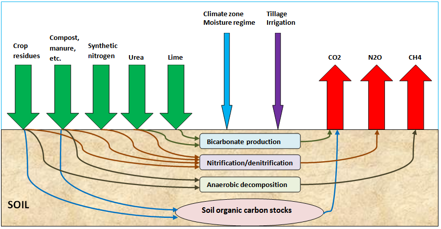
The diagram above captures the flow of key inputs into the soil and the resulting emissions of greenhouse gases (GHGs) as well as sequestration of soil organic carbon. The inputs of interest are synthetic fertilizers, organic fertilizers and soil amendments, and crop residues. The soil model basically tracks, to a first-order approximation, what happens to the nitrogen and carbon in these various inputs. The GHGs that are released as a result of these inputs, as well as due to land management practices and climatic conditions, are nitrous oxide (N2O), carbon dioxide (CO2) and methane (CH4).
How we model soil dynamics
Changes in soil organic carbon
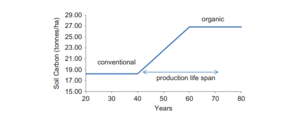
We use the IPCC tier 1 parameters (see discussion in the last section) to estimate changes to soil organic carbon (SOC) stocks in croplands. These parameters are a function of land management practices (tillage method, carbon inputs to soil), climate zone, moisture regime, and soil type. The default time period for stock changes is nominally 20 years and management practice is assumed to influence stocks to a depth of 30 cm. Soil carbon is considered to be in steady state until there is a significant land-use change (such as a conversion from grassland to cropland) or management change (such as a conversion from conventional cropland to organic cropland) that changes the soil carbon stocks.
When such a change occurs, the soil carbon is assumed to reach steady state again after 20 years under the new land-use or management practice. During this 20-year transition period, soil carbon may be increasing or decreasing each year as illustrated below, thus increasing or decreasing the total greenhouse gas emissions and the product carbon footprint during that period. When soil carbon is in steady state, it does not contribute to net emissions in agricultural systems.
Regarding the question of why a steady-state organic farming system does not get credit for the potentially higher level of carbon (relative to a conventional farming system) already accumulated in the soil: The addition of organic matter balances the carbon that is naturally oxidized away from the top layers of the soil, so in an ideal steady-state system, the SOC level remains constant and the net change in soil carbon is zero. LCA models account for this net change and a production system can take credit in the years that this net change > 0. Likewise, if we allowed the organic system to degrade by not adding sufficient organic matter to the soil for a few years, it would result in a new transition with net change < 0, resulting in a higher carbon footprint for those years. So maintaining a steady-state organic system avoids this higher carbon footprint — and that in a nutshell is the benefit of continuously adding organic matter to the soil. That benefit is already reflected in the stable carbon footprint of a steady-state organic system.
The 20-year transition period itself is not a critical parameter. Our tools allow the user to set this to any reasonable value. The more important issue is the magnitude of changes to the SOC stocks over the transition period. There can be wide variability and crop specificity in field measurements of soil carbon stocks, and the tier 1 parameters provide useful estimates of typical SOC changes while avoiding the complexity and data collection effort associated with tier 2/3 models.
Nitrous oxide emissions due to nitrogen inputs
Synthetic nitrogen fertilizers (nitrate, ammonia, ammonium or urea) and organic nitrogen sources (compost, manure or crop residues) produce direct N2O emissions from the soil through the nitrification-denitrification process mediated by soil bacteria. In addition, indirect N2O emissions result from the volatilization and redeposition of NH3/NOx, and through leaching and runoff of nitrogen.
We calculate both direct and indirect N2O emissions based on the amounts of synthetic and various organic nitrogen sources added to the soil each year, as well as due to nitrogen from crop residues and distinguishing between typical agricultural soils and flooded rice fields. We also make an adjustment for legumes to account for the excess ammonium that may leak from nitrogen-fixing root nodules and ultimately escape to the atmosphere as N2O.
Carbon dioxide emissions due to lime and urea
CO2 is released directly due to the application of lime and urea to agricultural soils. Liming is used to reduce soil acidity and improve plant growth. When carbonates such as limestone (CaCO3) are added to soils, they dissolve and release bicarbonate (HCO3-) which evolves into CO2 and water. When urea is applied as a fertilizer, it releases bicarbonate which again evolves into CO2 and water. We calculate these CO2 emissions based directly on the amounts of lime and urea applied each year to a given land area.
Methane emissions from rice fields
Anaerobic decomposition of organic material in flooded rice fields produces CH4. We calculate the annual amount of CH4 emitted from a given area of rice as a function of the crop growth period (measured in days), irrigation method (such as continuously or intermittently flooded), and organic and inorganic soil amendments (such as straw, compost and/or manure).
What the standards say
IPCC guidelines
The IPCC guidelines for national greenhouse gas inventories provide the most detailed and standardized guidance available for calculating soil carbon emissions and sequestration, N2O emissions from soils, and CH4 emissions from soils. Given that the current product carbon footprint standards do not provide detailed guidance on these topics but defer to IPCC in general, our methodology for modeling soil dynamics is based almost entirely on the IPCC guidelines.
There are three tiers of methodology in the IPCC guidelines. We have found the tier 1 methods to be the most appropriate for LCA models used to compute product carbon footprints. Given the time and cost constraints in most LCA projects, as well as the sheer difficulty involved in obtaining country-specific data or field measurements, we use tier 1 methods as a practical default unless higher tier data are readily available.
Here is a brief description of the three tiers:
Tier 1 methods are designed to be the simplest to use, for which equations and default parameter values (e.g., emission and stock change factors) are provided by IPCC. Country-specific activity data are needed.
Tier 2 can use the same methodological approach as Tier 1 but applies emission and stock change factors that are based on country- or region-specific data.
At Tier 3, higher order methods are used, including comprehensive field sampling repeated at regular time intervals and/or GIS-based systems of age, class/production data, soils data, and land-use and management activity data, integrating several types of monitoring.
Product carbon footprint standards
Neither of the two leading product carbon footprint standards, PAS-2050 and the GHG Protocol Product Standard, requires soil carbon changes (due to changes in management practices such as tillage) to be included in the carbon footprint of agricultural products. The default is to exclude it, but both standards provide for ways to include it (in the case PAS 2050, it can be included in accordance with the standard’s supplementary requirements). Both standards do require direct land use change (such as conversion from grassland to cropland) to be included per IPCC guidelines, but indirect land use change is not included in the carbon footprints. Our methodology is consistent with both standards, and we do include the effects of both land management practices and direct land use changes.
PAS 2050 requires non-CO2 emissions (N2O, CH4) from soils to be assessed using the highest tier approach set out in the IPCC guidelines or the highest tier approach employed in the country in which the emissions are produced. The Product Standard does not provide specific guidance on this. Our methodology takes a compromise position here and defaults to using the IPCC tier 1 parameters to calculate these soil emissions.
Carbon registries
The methodology described here generally aligns with the principles developed by carbon registries (for example, the Climate Action Reserve’s Soil Enrichment Protocol) for allocating carbon credits based on soil carbon sequestration.
We partnered
with a US-based producer of organic, plant-based frozen desserts to test drive our
hybrid methodology for compiling a corporate greenhouse
gas (GHG) inventory. This is the partner company’s first GHG inventory,
intended to establish a baseline for annual emissions and a basis for
potentially offsetting those emissions.
The hybrid
methodology combines two kinds of life-cycle inventory data to quickly and
efficiently produce a GHG inventory using CarbonScope:
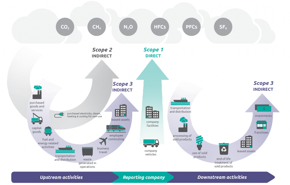
All of the emissions in scope 1 (direct
fuel combustion) and scope 2 (purchased electricity) are modeled using
our process LCI (PLCI) database,
which converts physical quantities of energy use into GHG emissions.
The company is classified as a small company (less than
100 employees and/or less than $50M in annual revenue). The company outsources
its product manufacturing to two co-packers both of whom are outside of the
company’s organizational boundary on an operational control basis, so the
entirety of the co-packer emissions will be categorized as scope 3.
Activity data
The company provided
activity data for this baseline inventory based on their operations in 2019,
using our standard data template for hybrid GHG inventories. The actual data is
confidential, but here is an example of what the input
data might look like for a hypothetical company. The activity data typically
includes:
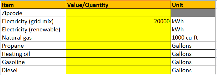
Fuel and electricity consumed in
company operations – in physical units such as kWh, gallons, etc.
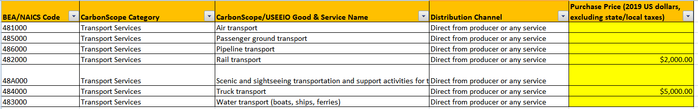
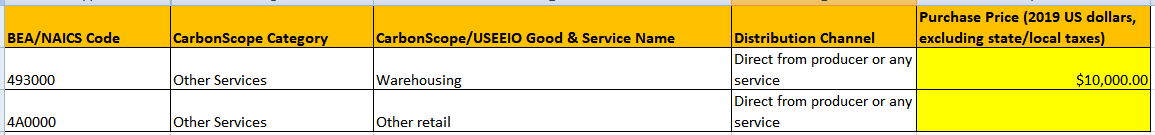
Goods and services purchased
(inflows) – in 2019 US dollars excluding taxes
Waste management services
purchased– in 2019 US dollars excluding taxes
Freight transport services
purchased– in 2019 US dollars excluding taxes
Warehousing and storage services
purchased– in 2019 US dollars excluding taxes
Energy used in processing and
use of sold products– in physical units such as kWh, gallons, etc.
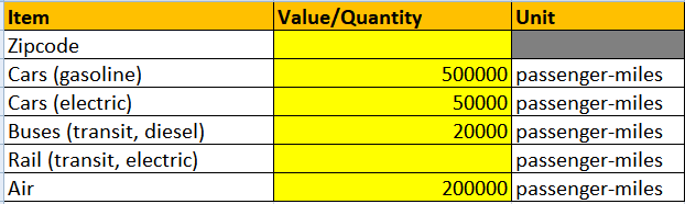
Employee travel and commuting—in
passenger miles or km
The larger of the two
co-packers was able to provide their detailed activity data separately. The
smaller co-packer was modeled as a supplier providing frozen dessert
manufacturing services within the company’s purchased goods and services.
The company sources 100%
of its electricity from renewable sources supplied by the local utility. The
larger co-packer produces about 3.2% of its electricity using on-site solar,
with the remainder sourced from the local grid.
Some of the plant-based ingredients
used in the dessert products are imported, which are modeled using domestic
production as proxy by assuming that imported commodities have the same input
structure and the same production characteristics as comparable products of
equal value produced domestically (see this methodology note). While all of the purchased ingredients are organically
produced, the inventory uses emission factors for industry sectors as a whole
without distinguishing between conventional and organic production. This can be
justified by the fact that organic farming does not necessarily have lower
carbon footprints than conventional farming when systems are in steady state.
Inventory results
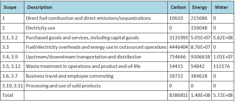
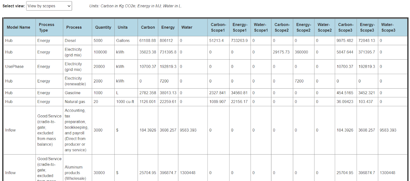
The results of the GHG inventory analysis show that the company’s operations from all three emission scopes amount to 8387 metric tonnes of CO2e for the year 2019. The table and chart below show a detailed breakdown (units: Carbon in Kg CO2e; Energy in MJ; Water in L).
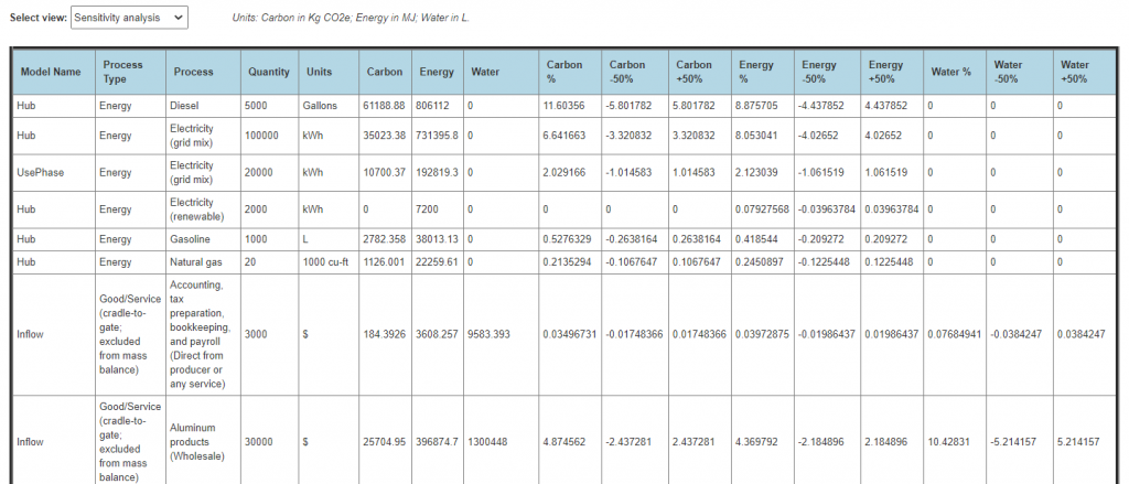
A sensitivity analysis shows that the natural gas used by the larger co-packer is by far the largest contributor to the corporate GHG emissions, accounting for 49% of the total emissions and reported under scope 3.3. The next four contributors are the ingredients sourced by the larger co-packer (16.6% of total emissions; scope 3.1), manufacturing services provided by the second co-packer (9% of total emissions; scope 3.1), truck transport services used to ship finished products (7.6% of total emissions; scope 3.9), and cardboard containers used to ship finished products (3.8% of total emissions; scope 3.1). Overall, scope 3 emissions account for over 99% of the total emissions and 72% of the total emissions are attributable to the larger co-packer.
For a hypothetical
company with revenue at the midpoint of the range for the company size, the GHG emissions intensity is 0.36 Kg CO2e
per dollar of revenue. This intensity is less than 50% of industry average for
the ice cream and frozen dessert sector in the US.
Effort
We said at the outset
that our hybrid methodology provides for a quick and efficient way to compile a
corporate GHG inventory. Here is a quick
accounting of the time and effort that went into generating the inventory:
About 2.5 weeks of work by the
company’s sustainability team to collect activity data from within the company
and from the co-packers.
A few hours to automatically
import the data into CarbonScope, generate results, and review/interpret the
results.
With a baseline GHG
emissions inventory established using a simple and well-understood methodology,
annual updates to the inventory are expected to take less time/effort and turn
into a routine accounting task.
Think before you drink: The carbon footprints of four different hydration options
Susan Cholette and Hoa Nguyen
Project summary
Hydration
is a necessity, and the growing consumer shift away from soft drinks towards
water should please dentists and physicians alike. However, as worldwide demand has surpassed
half a trillion bottles per year, single use plastic bottles are not the healthiest
choice for the planet. We compare
several scenarios for quenching thirst on the go, and show how our purchasing
habits can make a substantive impact.
Systems modeled in this study
We evaluate
four different ways to provide a thirsty Bay Area consumer a half-liter of
water: imported bottled water, more locally
sourced water bottled in both virgin and 100% recycled PET bottles, and a
reusable container that can be refilled as needed.
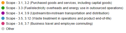
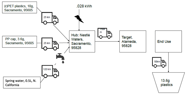
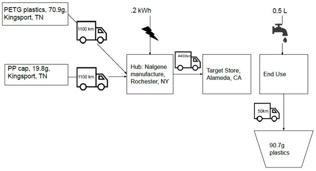
The following figures illustrate the supply chains for a 500ml bottle of Evian, imported from Switzerland, and Arrowhead™, which sources from Californian springs. According to their website all of Arrowhead™’s individually sized bottles sold in California are currently comprised of a 50/50 mix of virgin and recycled PET, but they indicate their bottle design can support use of 100% recycled content and will eventually. Some other drink companies, such as Snapple™ have recently re-designed their bottles to use 100% recycled content. We consider both extremes for recycled content- 0% and 100%- to illustrate the relative impact that recycling has, and we assume that the recycled PET is sourced from the same location as virgin PET.
Figure 1: System diagram for a 500ml bottle of Arrowhead™ water
Figure 2: System Diagram for a 500ml bottle of Evian™ water
While consumers have many options for reusable containers, we select a Nalgene™ bottle to keep within the same family of materials, as it is made of Tritan™, a popular form of PETG plastic. Unlike the prior three scenarios, where the functional unit is a half liter bottle of water, the functional unit is just the Nalgene™ bottle itself, as it is purchased empty and then filled at home or at a drinking fountain, as shown in Figure 3. We assume that no additional filtration or treatment is used.
Figure 3: System diagram for a Nalgene™ reusable container
All four
scenarios share the same system boundary,
cradle-to-grave, where we assume that the bottles are trucked to landfill once
discarded, as only about 30% of plastic containers are recycled in the US.
LCA tool and LCI database
We used our carbon modeling tool, CarbonScope, to conduct the LCAs in this project. The life-cycle inventory (LCI) database underlying the analysis is CarbonScopeData.
Results
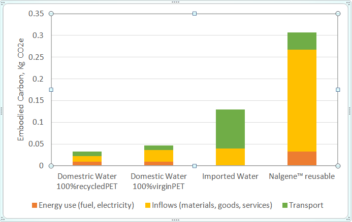
The three life-cycle impact categories that can be quantified are embodied carbon (kg CO2e), embodied energy (MJ) and embodied water (L), but to keep the comparisons simple, we report only embodied carbon. Other studies published elsewhere discuss the additional problem of landfill usage and pollution from bottles that escape proper disposal.
Figure 4 shows the relative impacts of each of the bottles and the contribution for each stage towards embodied carbon. The domestically sourced water bottled in 100% recycled PET has the lowest footprint, a 30% reduction over the virgin PET bottle. Imported water has almost three times the footprint, thanks to the international transportation required. Figure 4 also shows that distance trumps recycled content: even if we were to buy an imported brand bottled in 100% recycled materials, it is clear that it would have more embodied carbon than the domestic water bottled in virgin PET. The reusable container has the most embodied carbon due to its greater weight, more energy-intensive material, and the need to transport it across the country.
Figure 4: Embodied carbon associated with a single use of each of the four bottles
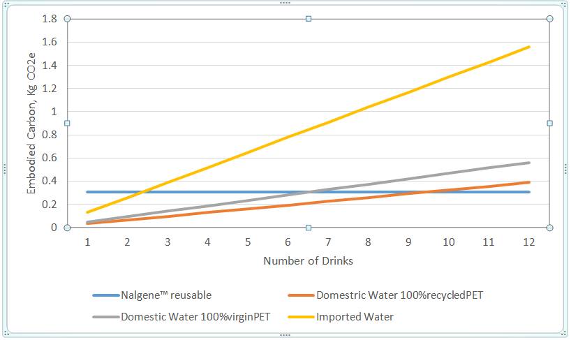
Of course, it would be silly to purchase a reusable container for one time use. Figure 5 illustrates the how cumulative carbon footprint increases with the number of uses. We include the .001 kg CO2e associated with pumping and treating tap water, a miniscule impact that effectively results in a flat line for the Nalgene™ reusable bottle no matter how many times it is refilled.
Figure 5: Cumulative GHG Impact: Consumption of 500ml of Water
The initial investment in a reusable bottle pays off quickly: we need only use it three times over the purchase of imported water to accumulate less embodied carbon. We would need to reuse a Nalgene™ bottle just more than six or nine times to have a lower footprint than domestically sourced water bottled in virgin or recycled PET. Given that such containers sell for $10 or more, it is likely that we would break even environmentally before we do financially.
While metal or glass containers will have different footprints, the environmental benefit of using reusable drinking containers will be even more advantageous than it is for shopping bags, with one study showing it may take more than 170 uses to offset the investment in a cotton bag over the typical HDPE bags provided at checkout. This is understandable since the transportation of water is inherently emissions intensive. For example, even though the domestic water is sourced from relatively nearby springs, the transport of the water comprises over 20% of the total footprint, while the pumping and treatment of the water is less than 1%. Other domestic brands that use out of state water sources will have a higher transportation footprint.
Conclusions
In summary, the best choice for hydration is to develop a habit of bringing along a reusable container. If that is not an option, then buy a brand of bottled water that is more locally sourced, as distance has a larger impact than the percent of recycled content in the bottle. Imported water should be consumed sparingly, regardless of how it is packaged. Thankfully, imported bottled water has a small and shrinking share of the overall market for still water: only one brand (Fiji) is represented in the top brands that comprise 75% of the US market, and it has a small (3%) share.
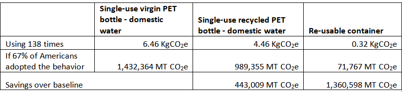
Table 1: What-if analysis for alternate purchasing behavior
Americans currently purchase an average of 36.5 gallons of bottled water annually, about 275 500ml bottles. While some purchases of single-use water bottles may be necessary, if 200 million Americans obtained a reusable container and replaced half of their yearly bottled water purchases by refilling these containers at taps or drinking fountains, Table 1 shows we could avoid over 1.3 million metric tons of CO2e emissions annually. While this represents only 0.025% of the national annual emissions, this would be a relatively painless behavior to adopt. Small drops do add up.
As app developers, our primary focus at CleanMetrics has been on tools and apps that businesses and organizations can use to quantify, track and reduce their climate impacts.
We have been increasingly hearing from other app developers looking to integrate a life-cycle inventory (LCI) database with their consumer-facing apps. These apps typically let consumers track their personal carbon emissions from purchases and other activities. The idea is to help consumers become climate-savvy in their purchasing decisions and/or make it easy for them to offset their emissions.
We are now releasing an API to our LCI database, CarbonScopeData, to address the lack of high-quality carbon emissions data that plagues many consumer-facing apps. We want to help improve the quality of climate and carbon apps across board, and thereby empower consumers to take decisive action to slow climate change.
The CarbonScopeData API is a RESTful web service that provides access to both process LCI and environmentally extended input-output LCI data.
The process LCI dataset contains over 1400 materials, products and processes, including the largest commercially available LCI database for North American food production and processing. The input-output LCI dataset uses data on economic transactions between industry sectors to provide life-cycle data for 385 US goods and services covering the entire US economy.
The database provides three key life cycle metrics: greenhouse gas emissions (embodied carbon), primary energy use (embodied energy) and water use (embodied/virtual water).
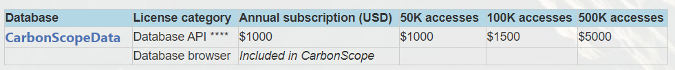
As usual, our pricing structure is designed to reduce barriers and make emissions accounting as widespread as possible. We require an annual subscription and purchase of API accesses sold in blocks of 50,000/100,000/500,000 accesses.
An annual corporate greenhouse gas (GHG) emissions inventory – if done correctly – can tell you exactly where your company or organization stands as far as its climate impact and how that changes over time. It is a starting point for serious climate action that could ultimately include switching to green electricity, cutting transport emissions, using lower-emissions materials, reducing waste and purchasing high-quality carbon offsets.
But GHG inventories are notoriously time-consuming and difficult to compile, and they often require a level of expertise that most small and medium-sized enterprises do not have. This problem was front and center in our minds as we architected and developed our new carbon modeling tool, CarbonScope. As we said in a recent Medium post: If we are going to bend the emissions curve, then a majority of businesses need to get involved, and emissions accounting must become as commonplace as financial accounting.
While CarbonScope allows for some very sophisticated modeling, we want to focus here on the simplest and quickest way to compile a corporate GHG inventory that you can put to use immediately. CarbonScope is a web app designed for interactive data input and use. To keep things simple, we will propose entering all of the activity data into a spreadsheet and then uploading it into CarbonScope. Once the data is in CarbonScope, you can switch to an interactive mode for the rest of the analysis.
This simple method uses hybrid life-cycle inventory (LCI) data under the hood:
All of the emissions in scope 1 (direct fuel combustion) and scope 2 (purchased electricity) are modeled using our process LCI (PLCI) database. This is the easy part.
The wide range of emissions in scope 3 are modeled largely using our environmentally extended input-output LCI (EEIOLCI) database, which converts dollar amounts from purchase records into equivalent GHG emissions, energy use and water use based on the industry sector (or equivalently, NAICS code). This is the difficult part that we have simplified and automated to a large extent.
This hybrid method is available to companies that are using CarbonScope themselves, as well as to those that utilize our consulting services.
Compile activity data
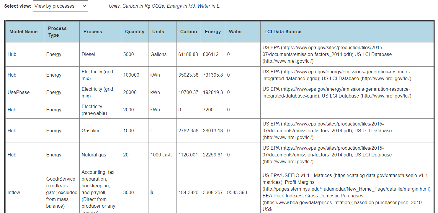
We have an example of the activity data template here with some sample data filled in for a hypothetical company. Note that this data is for a one year period. The spreadsheet contains seven sheets:
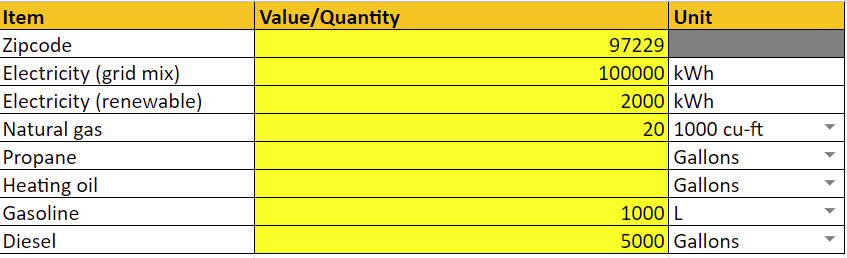
Hub: This is the company’s primary location (or it could be the location of a division, subsidiary or department). Here we would fill in the quantities of all purchased fuels and electricity, accounting for all of the scope 1 and 2 emissions (and some scope 3 emissions as well). A zipcode is required in order to find the correct electric grid emission factor in the US (alternately, you can enter a country name here for international locations). A blank zipcode defaults to US average electric grid emissions.
Inflow: This sheet captures all of the purchased materials, goods and services. The cool thing about this is that CarbonScope can work with dollar amounts (excluding local/state taxes) that you spent on your purchases from one or more of 385 industry sectors that cover the entire US economy. You can just convert your purchasing records into dollar amounts that can be used to represent most of the scope 3 emissions, resulting in significant savings of time and effort.
Outflow: This sheet captures all of the third-party freight transport that you paid for. It is also in dollar amounts similar to the inflow. This contributes to scope 3 emissions.
Waste: This sheet captures all of the waste management, water and wastewater services that you paid for. It is also in dollar amounts similar to the inflow. This contributes to scope 3 emissions.
Storage: This sheet captures all of the third-party warehousing or other storage of your products that you paid for. It is also in dollar amounts similar to the inflow. This contributes to scope 3 emissions.
Use Phase: This sheet captures the estimated electricity and fuels consumed in the usage of your products, or in the further processing of your products in the value chain. This contributes to scope 3 emissions. A blank zipcode defaults to US average electric grid emissions.
Employee Travel: This sheet captures all of the employee business travel and commuting in passenger miles on various transport modes. It is the total across the entire company (or division, department, etc.). This contributes to scope 3 emissions. A blank zipcode defaults to US average electric grid emissions.
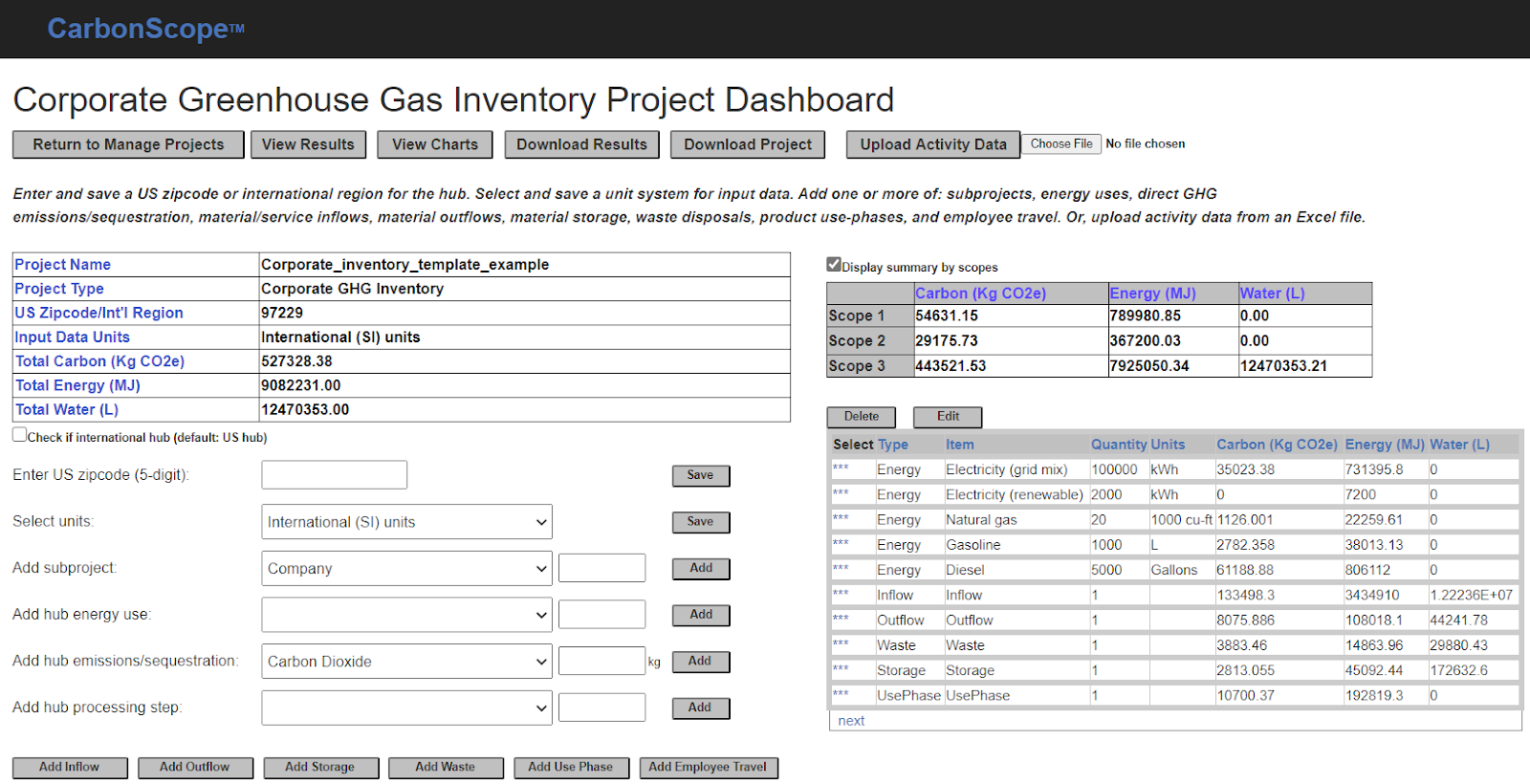
Upload activity data
This spreadsheet with its seven sheets can be uploaded into a blank GHG inventory project in CarbonScope by selecting the Excel file and clicking “Upload Activity Data” in the CarbonScope GHG inventory dashboard. The upload will automatically populate the project and calculate all of the carbon, energy and water results in detail. At this point, all of the analysis is automatically done and summary results can be seen on the dashboard as shown below. It is as simple as that.
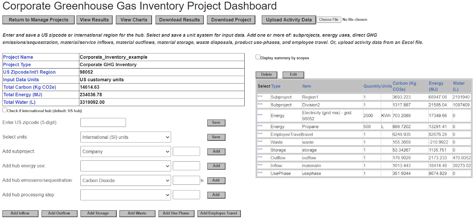
Note: If the company has multiple locations, divisions or subsidiaries that need to be modeled separately, you would need to fill out one copy of the spreadsheet for each of these and upload each spreadsheet into a separate GHG inventory project. Then, you would instantiate these other projects as subprojects within the GHG inventory project for the main location or the company headquarters as shown below.
View and download results
The full GHG inventory results can be downloaded by clicking “Download Results” on the dashboard. You can see the results for the above hypothetical example here. You can slice and dice the results as needed, and create your own custom reports.
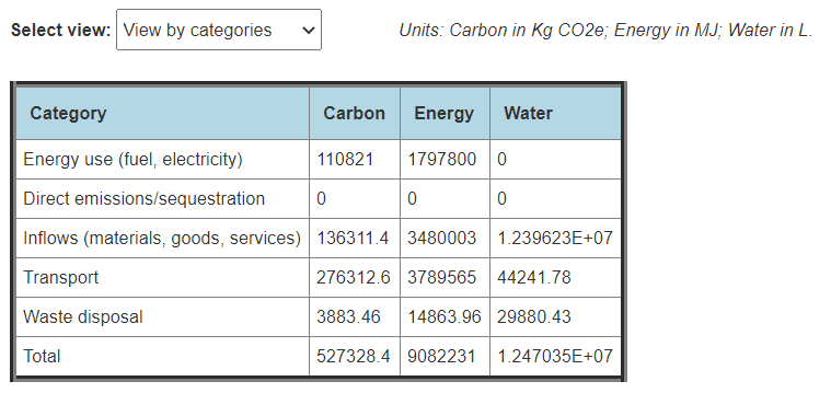
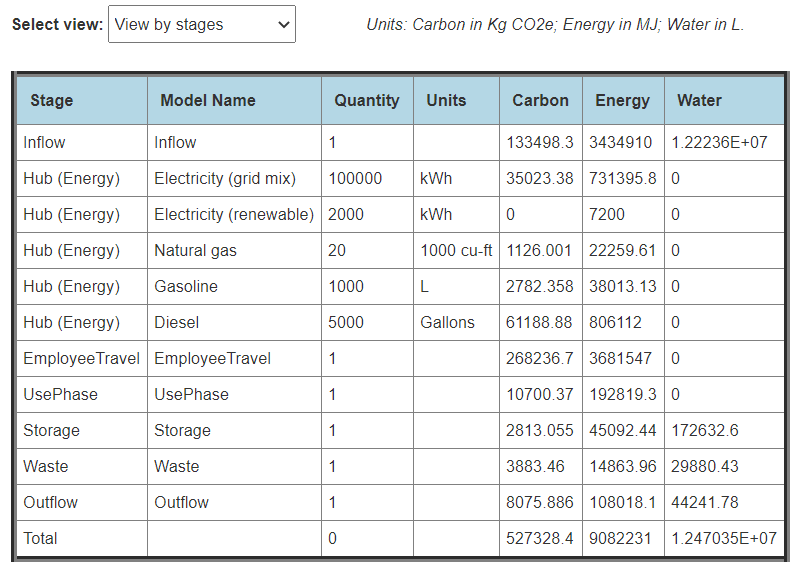
The same basic results can be viewed online by clicking “View Results” (to view as tables) or “View Charts” (to view as charts) on the dashboard and then selecting the desired “view” in the new browser tab that opens up. The results can be viewed by category, stages, processes or scopes as shown below. A sensitivity analysis table is also available.
View by categories ______________________________________________________________________View by stages ______________________________________________________________________View by processes _____________________________________________________________________View by scopes _____________________________________________________________________Sensitivity analysis ______________________________________________________________________
Correct usage of the hybrid methodology
The hybrid methodology outlined here — combining PLCI (for accurate scope 1/2 emissions and some scope 3 emissions) and EEIOLCI (for 100% coverage of most scope 3 emissions) — can be very effective in compiling corporate GHG inventories.
A limitation of EEIOLCI is that it cannot be used for evaluating the relative impacts of process improvements or material substitutions within an industry sector, or for comparing the environmental impacts of two similar products, due to the data aggregation by industry sector.
This hybrid methodology can be used to quickly establish a baseline GHG inventory and can help screen for hot spots that may require more attention. Emission reduction targets can be set immediately for scopes 1 and 2 in accordance with Science Based Targetsor other reduction plans. The inventory results can also be used directly to purchase high-quality carbon offsets as part of a broader corporate climate strategy to address all emission scopes.
With the sensitivity analysis that CarbonScope performs automatically, it is straightforward to identify the scope 3 items that the GHG inventory is most sensitive to. Based on this, some of the scope 3 items (especially the inflows of goods and services into the company/organization) could be selectively modeled using PLCI in a second iteration for more accuracy as well as to evaluate process improvements or material substitutions in order to set and achieve scope 3 emission reduction targets. Alternately, it might be useful to look at categories like employee travel for possible scope 3 emission reductions while keeping the convenient EEIOLCI modeling for inflows.